ОБЗОРЫ - Моделирование сигнальных процессов в современном HDD

Представляем вам материалы от компании ChannelScience — одной из ведущих исследовательских компаний в области теории магнетизма, кодирования и сигнальных процессов в современных магнитных носителях информации. Моделирование процессов представляется на примере специального мощного ПО — PRMLpro™, предназначенного для исследования, различных экспериментов и моделирования процессов из области теории сигналов.

Возможности PRMLpro™ включают в себя полную эмуляцию всех стадий обработки аналогового сигнала, полученного со считывающего элемента головки HDD до финального результата — декодированной и ECC-откорректированной битовой последовательности паттерна данных, т. е. 512 байт информации, записанной в секторе, осциллограмма которого обрабатывалась. В качестве исходного сигнала можно задать *.WAV файл, который, в свою очередь, можно «сграбить» с помощью специального электронного оборудования. В качестве примера можно привести Disk Drive Analyser от компании Teledyne LECROY — DDA5005A либо его топовый современный аналог DDA 760Zi-A: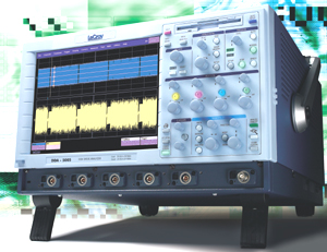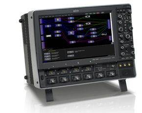

Аппаратура подобного класса входит в подгруппу приборов, называемых High Definition Oscilloscopes. Подробное описание и технические характеристики можно посмотреть здесь.

Описание теории и алгоритмов работы PRML-декодера предоставлено Александром Тараториным, физиком-исследователем из США. Также им выпущена книга "Characterization of Magnetic Recording Systems: A Practical Approach", в которой максимально подробно описываются алгоритмы работы узлов современного HDD. Стоимость книги — 85 $.

Вследствие большого объёма текстового материала, а также его узкой технической направленности и многочисленных графических иллюстраций (скриншотов программы) мы не стали переводить его на русский язык и предоставляем читателю оригинальный текст.

1. Building a data sector
1.1 What is in a data sector?
1.2 Specifying a data sector in PRMLpro™
1.3 Scrambler
1.4 RLL Encoder
1.5 Precoder
1.6 Save Results
1.7 Save Settings

2. Creating a Modeled Waveform
2.1 Load binary input pattern
2.2 Apply additional precoding
2.3 Select pulse models
2.4 Apply media noise
2.5 View and save the waveforms
2.6 Save Settings

3. Noise and Distortion
3.1 Load a PRMLpro™ Waveform
3.2 Add White Gaussian Noise
3.3 Add Colored Gaussian Noise
3.4 Add Thermal Asperities
3.5 Save Results
3.6 Save Screen

4. Filter the Noisy Waveform
4.1 Load Noisy Waveform
4.2 Adjust Filter Settings
4.3 Filter Other Waveforms
4.4 Save Results
4.5 Save Screen

5. Detect the Data
5.1 Load Clean Waveform as Reference
5.2 Adjust Viterbi Algorithm Settings
5.3 Process Reference Waveform
5.4 Load Noisy Filtered Waveform as Comparison
5.5 Process Comparison Waveform
5.6 Save Results

Building a data sector

What is in a data sector?

The typical hard disk drive sector consists of four parts: Preamble, Sync, Encoded User Data, and Pad. The preamble is a single frequency pattern that is used by the automatic gain control (AGC) and phase-locked loop (PLL) to establish initial gain and timing. The detector also uses the preamble to determine the correct initial state sequence.

The preamble is typically a 2T pattern. Here "T" means one channel clock period. For example, a 1Gbps channel rate translates into 1ns bit intervals (channel clock periods). In this case, a 2T pattern has a magnetic transition every 2ns. Because transitions alternate positive and negative, one complete period of a 2T pattern spans 4T, or 4ns in this example. The corresponding preamble frequency is 250MHz. The typical preamble spans about 48 to 120 channel bits.

The preamble is followed by a sync mark. This signals the end of the preamble and the beginning of the encoded user data. It typically spans 18 to 27 channel bits. Sometimes redundant sync marks are used.

The user data is most often a 512-Byte (4096-bit) block of binary data that has been scrambled and RLL (run-length limited) encoded. With a 16/17 rate code, the 4096 user bits are mapped into 4352 channel bits.

A pad of about 32 to 64 channel bits is often appended at the end of the sector to keep the data clocking through the channel and to resolve any ambiguous final code states.

Specifying a data sector in PRMLpro™

The Data Pattern Creation screen shown below opens when the corresponding button on the PRMLpro™ control screen is pushed. Notice that the four portions of the preamble are specified across the top of this screen. Editboxes are provided for entering the portion of the preamble and pad that will be repeated. The number of times to repeat each portion of the sector is specified at the right hand side of the screen under the heading "Occurs." For example, in the figure below, the preamble pattern (1010) is to occur 20 times. The resulting pattern spans 80 channel bits. The whole frame sync mark is usually specified in the editbox, so the number of occurrences is typically 1.

PRMLpro™ provides four ways to specify the user data portion of the sector. You may load in a file, saved in PRMLpro™ format. Note that PRMLpro™provides a file conversion utility that should make most common file formats compatible with PRMLpro™. You can access the File Conversion Screen from the corresponding pushbutton on the Control Screen.

You may also manually type in a desired data pattern. Further, two automatic pattern generation methods are provided. Both are based on pseudo-random binary sequences (PRBSs). The equiprobability option generates a user-specified number of 1s and 0s. The occurrence of a 1 or 0 is equally likely (0.5). You may specify the starting seed for the underlying pseudo-random number generator. This enables you to re-create the same "random" pattern by using the same seed.

The most common choice for specifying the data pattern is the PRBS option. This produces similar results as the equiprobability option, except you have control over the exact pseudo-random binary sequence that is created. This control is exercised by specifying the linear feedback shift-register (LFSR) that is used to create the sequence. The PRMLpro™ default settings for the polynomial that specifies the LFSR follow the popular suggestions of Peterson and Weldon and of Bergmans.

Remember, you must push "Display Now" before any changes that you make on the screen will take effect.

The input to the editboxes for preamble, frame sync, pattern and pad must be 1 and 0s only. These binary sequences must not include SPACES or any other characters. For example, use 11000011 NOT 1 1 0 0 0 0 1 1. In contrast, editboxes for "Polynomial" and "Initial States" MUST include spaces. For example, 1100 would be interpreted as one thousand one hundred in these editboxes, instead of the intended 1-1-0-0. The only exception to these conventions is when the "Non-Bin" (non-Binary) button is used with the "Manual" pattern option. Specifically, you may enter a non-binary pattern, such as +3.52 -2.01 0 1.52, into the manual editbox. Note the use of spaces. Then push Non-Bin to write a PRMLpro™ file with these values. This is useful for creating small sequences of sample values for FIR or Viterbi experimentation.

Assume an NRZI interpretation of the binary patterns. That is, a 1 indicates a transition and a 0 indicates no transition. Then, in summary, the settings in the figure above will create the following "Original Pattern" when "Display Now" is pushed. The pattern begins with a 2T preamble pattern that spans 80 channel bits ( = 4 * 20). Then a 17 channel bit sync mark is inserted. This is followed by 511 pseudo-random user bits. Finally 40 channel bits of 2T pattern are appended as the pad.

Clicking the "Original Pattern" radiobutton beside either plot at the bottom of the Data Pattern Creation screen causes the pattern to be plotted as a sequence of 1s and 0s. The 1s and 0s are also displayed in the textbox between the graphs. The spectrum of this sequence is displayed (in the corresponding color blue or red) in the plot at the extreme right of the screen. Any graph can be zoomed in on by dragging a box on it. Further any graph can be enlarged and opened in a separate window by right-clicking on the graph and selecting "Open in New Window" from the context sensitive pop-up menu.

WARNING: It is important to test your channel and simulations with many different pseudo-random sequences. Failure to do this may mask the presence of important problems such as missed sync marks due to interactions with certain data patterns that might immediately follow the sync pattern.

Scrambler

The user data is typically scrambled by XORing it with a PRBS. This has the desirable effect of breaking up repetitive patterns in the user data. The spectrum of the scrambled user data is typically more "white" than unscrambled user data. This is not the case if the user data itself was simulated as a PRBS. In this case, the unscrambled spectrum is already white. PRMLpro™ only scrambles the user data pattern — not the preamble, sync or pad. Remember, you must push "Display Now" before any changes that you make on the screen will take effect.

As an example,the settings in the figure above will create a PRBS based on the scrambler polynomial and initial conditions. This sequence is XORed with the data pattern only. The resulting sequence of preamble, sync, scrambled user data and pad is plotted when the radiobutton beside "Scrambled" is pushed. The sequence is also displayed in the textbox between the graphs. The spectrum of this sequence is displayed (in the corresponding color blue or red) in the plot at the extreme right of the screen. Any graph can be zoomed in on by dragging a box on it. Further any graph can be enlarged and opened in a separate window by right-clicking on the graph and selecting "Open in New Window" from the context sensitive pop-up menu.

RLL Encoder

Run-length limited encoding maps the user data into a new, longer sequence. This sequence follows the d, k run-length constraints of the code. Specifically, the encoded sequence does not have fewer than d 0s between 1s and no more than k 0s between 1s. Some codes also have an interleave k constraint, k-int. This means that both the even and odd bit sub-sequences have no more than k-int 0s between 1s.

PRMLpro™ applies RLL encoding to the scrambled user data and the pad. Some RLL codes look-ahead to the next bits in order to determine how to encode the current bits. The pad is encoded so that a group of bits at the end of the scrambled user data never results in an ambiguous encoding state.

In the figure above, a 16/17 rate RLL code is used. This takes 16 user bits and maps them into 17 code bits, or channel bits. Note that d=0, k=12 and k-int=8. This means that the encoded sequence can have 1s right next to each other, but there will be no more than 12 0s between 1s. Further, looking at every other bit (the odd or even bit sub-sequence), there will be no more than 8 0s between 1s in each sub-sequence.

Remember, you must push "Display Now" to see the effects of any changes you make to the screen settings.

The resulting sequence of preamble, sync, RLL encoded scrambled user data and RLL encoded pad is plotted when the radiobutton beside "RLL Encoded" is pushed. The sequence is also displayed in the textbox between the graphs. The spectrum of this sequence is displayed (in the corresponding color blue or red) in the plot at the extreme right of the screen. Any graph can be zoomed in on by dragging a box on it. Further, any graph can be enlarged and opened in a separate window by right-clicking on the graph and selecting "Open in New Window" from the context sensitive pop-up menu. Note that in the spectrum plot, the maximum frequency, 0.5, corresponds to the channel (or code) rate. That is, it corresponds to the rate at which the code bits pass through the channel. This is faster than the rate at which the user bits are passed between the read channel and the controller.

Precoder

The entire data sector (preamble; sync mark; RLL encoded, scrambled user data; and RLL encoded pad) is precoded. Popular PRML precoders are 1/(1 XOR D) and 1/(1 XOR D2). These and other precoders are preset into PRMLpro™. You can also specify a custom precoder numerator and denominator. The initial conditions for both the precoder input and output are usually all 0s.

Remember, you must push "Display Now" to see the effects of any changes you make to the screen settings.

The resulting sequence of precoded preamble, precoded sync, precoded RLL encoded scrambled user data and precoded RLL encoded pad is plotted when the radiobutton beside "Precoded" is pushed. The sequence is also displayed in the textbox between the graphs. The spectrum of this sequence is displayed (in the corresponding color blue or red) in the plot at the extreme right of the screen. Any graph can be zoomed in on by dragging a box on it. Further any graph can be enlarged and opened in a separate window by right-clicking on the graph and selecting "Open in New Window" from the context sensitive pop-up menu. Note that in the spectrum plot, the maximum frequency, 0.5, corresponds to the channel rate. That is, it corresponds to the rate at which the code bits pass through the channel. This is faster than the rate at which the user bits are passed between the read channel and the controller.

Save Results

The "Save Results" pushbutton saves the last patterns that were created. To make sure you are saving the exact patterns that you intend, it is good practice to always push "Display Now" JUST BEFORE saving your results. In the file dialog box that opens, type in a name for the files. The name you type will be used as a prefix for all of the files that are saved. Each file's name will have an identifying string appended that indicates which pattern it contains and that it was saved by the waveform creation screen.

Warning: File names must not contain spaces or other restricted characters and should be no longer than 32 characters (including the extension).

"Save Results" saves information from the Data Pattern creation screen in two formats. First the vectors corresponding to the original, scrambled, encoded and precoded sequences are all saved as a MATLABR workspace. To load this file into MATLABR, type the following in the MATLABR command window:

>> load filename.dpo -mat

When filename.dpo is loaded into MATLABR, all of the variables are placed into the MATLABR workspace.

Each of these vectors is also saved individually in its own file. These files have the ".dpo" extension, too. They are saved in MATLABR format, as if they had a ".mat" extension. These individual files load directly into other PRMLpro™ screens. Further, you can use the File Conversion utility to translate the .dpo format into ASCII. This universal format can be read into spreadsheets or word processors for manipulation. Most programs have a way to accept ASCII files or have a way to convert them.

Save Settings

The "Save Settings" pushbutton saves the entire Waveform Creation Screen as displayed. It also saves all of the internal variables that you have loaded and/or calculated in the screen. In the file dialog box that opens, type in a name for the saved screen. Usually this name is chosen to indicate the project with which you want to associate the screen. The name you type will be used as a prefix for the saved file. The string "_ptd.fig" is appended to indicate that the file is a Waveform Creation screen.

Warning: File names must not contain spaces or other restricted characters and should be no longer than 32 characters (including the extension).

This feature saves you time because you do not have to re-enter channel settings each time you use PRMLpro™. Saving screen settings is also very useful for sending extremely detailed information throughout your company and to customers and suppliers.

Creating a Modeled Waveform

Load binary input pattern

The Waveform Creation screen creates waveforms that correspond to stored binary data patterns. The screen accepts a file that represents the stored binary data. This file contains 1s and 0s that you can specify to be interpreted as NRZ or NRZI patterns. Three different pulse models may be used simultaneously to create three different waveforms. Media noise (transition jitter) may be applied to all three waveforms, provided NRZI mode is used.

To load a binary input pattern, press the "Load Binary Input" pushbutton in the upper right hand corner of the Waveform Creation screen. Browse for a PRMLpro™ (*.dpo) file to use. This file should contain a vector of 1s and 0s. If you downloaded the "Examples" files, load file c:\PRMLpro\Examples\511_original.dpo to use as an example. The results of this operation are shown below.

The file is displayed as a stem plot in the top graph. Notice that the file name appears in the graph title. Two radiobuttons above the graph allow you to select how the 1s and 0s are interpreted. NRZI mode is the most versatile. In NRZI mode, a 1 indicates the presence of a transition; a 0 indicates no transition. Further, the Waveform Creation screen automatically alternates the polarity of the 1s (transitions). NRZ mode interprets 1s as positive polarity write current and 0s as negative polarity write current.

To refresh the binary pattern stem plot, press the "Display Binary Input" pushbutton. Any graph can be zoomed in on by dragging a box on it. Further, any graph can be enlarged and opened in a separate window by right-clicking on the graph and selecting "Open in New Window" from the context sensitive pop-up menu.

Apply additional precoding

If you find that the data pattern that you have loaded is not in the correct form, you may precode it. To enable precoding, click the checkbox beside "Additional Precoding." Specify the numerator and denominator of the precoder transfer function in increasing powers of D. For example, the common 1/(1 xor D^2) precoder is specified as Numerator = 1 and Denominator = 1 0 1 — that is 1*D^0 + 0*D^1 + 1*D^1. This precoder exclusive ORs the current input with its output from two time instants earlier.

Initial conditions for precoding are usually set to all zeros. However, you can enter whatever binary pattern you wish. The numerator uses initial INPUT conditions. The denominator uses initial OUTPUT conditions. The number of elements you will need for the numerator or denominator initial conditions equals one less than the order of the corresponding polynomial. For the 1/(1 xor D^2) precoder example above, you will need no initial input conditions for the numerator, but you will need two initial output conditions (e.g., 0 0) for the denominator.

Note: Extra spaces between 1s and 0s are interpreted as additional 0s under some circumstances. To be sure you are always getting the precoding you intend, use EXACTLY ONE space between binary coefficients.

To see the results of your precoding, refresh the binary pattern stem plot by pressing the "Display Binary Input" pushbutton.

Select pulse models

A very useful and powerful feature of PRMLpro™ is the ability to quickly, easily and simultaneously create waveforms using target, standard and custom pulse models — all representing the same stored binary pattern.

Click the checkbox beside "Sinc Response" to create a target pulse response using sinc (sin(x)/x) functions. Several standard target pulses, such as EPR4, are already built in. A waveform is constructed that exactly hits your desired target values every "OSR" time steps (Note, OSR, the OverSampling Ratio, is commonly set to 10 samples between data bits). Sinc functions are used to fit a minimum bandwidth continuous-time waveform between the target samples.

When you push "Display Now" the waveform is calculated and displayed in blue. The Impulse (di-pulse) response is used in NRZ mode. An impulse is placed at every 1 in the binary input pattern. At every 0, -1 times the impulse response is used. In NRZI mode, a Positive Pulse is placed at the odd 1s. A Negative Pulse is placed at the even 1s. No pulses are placed at the 0s. We recommend always creating a waveform based on the sinc response. This waveform provides the ideal target sequence for data-directed LMS adaptation and for use as a reference sequence during Viterbi detection.

Click the checkbox beside "Model Response" to create a pulse response using popular pulse models such as the Lorentzian and the Gaussian functions. The maximum value of all native PRMLpro™ pulse models is +1. Change the pulse peak amplitude by changing the value of "Gain" from 1. Specify the channel bit density ("cbd" or "Dchannel") as PW50/T (the pulse width at 50 % amplitude, divided by the channel bit interval — both are given in units of OSR). Typical densities for hard disk drives are about 2.5 to 3.5.

In the figure above, the model waveform is created using a mixed pulse that is 25 % Lorentzian and 75 % Gaussian. The peak amplitude of the isolated pulse is 2 and the PW50/T is 2. At an OSR of 10, this amplitude and density mean that there are exactly 20 ( = PW50/T * OSR) sample points in the isolated pulse, from one 50 % amplitude point to the other (1 is 50 % of peak amplitude).

Asymmetric waveforms are created by changing the ratios in the three editboxes below the "Asymmetries" heading. The first editbox adjusts leading vs. trailing pulse asymmetry. For example, entering 1.3 in this box creates a pulse whose leading side (before the peak) is 30 % wider than the trailing side (after the peak). Entering 1.25 in the Pos/Neg Amp editbox multiplies the amplitude of the positive pulse by 1.25, but the negative pulse is untouched. Similarly a 1.25 in the Pos/Neg PW50 editbox causes positive pulses to have 25 % wider PW50s than negative pulses.

When you push "Display Now" the model waveform is calculated and displayed in red. The Impulse (di-pulse) response is used in NRZ mode. Amplitude and PW50 asymmetries are not used in this mode. An impulse is placed at every 1 in the binary input pattern. At every 0, -1 times the impulse response is used. In NRZI mode, a Positive Pulse is placed at the odd 1s. A Negative Pulse is placed at the even 1s. No pulses are placed at the 0s.

The waveforms created by using an EPR4 target sinc pulse and a 25/75 lor/gaus pulse with peak amplitude of 2 and density 2 is shown below. No asymmetries or media noise were applied.

It is also possible to create waveforms based on files that represent pulses. These files are typically generated by micro--magnetic models or captured from an oscilloscope. Usually the files will need to be resampled such that they have OSR samples per data bit interval. This is accomplished automatically when the editboxes for Data Rate, OSR and Sampling Frequency are filled out BEFORE loading a file response.

When you push "Display Now" the waveform is calculated and displayed in green. The Impulse (di-pulse) Response is used in NRZ mode. An impulse is placed at every 1 in the binary input pattern. At every 0, -1 times the impulse response is used. In NRZI mode, a Positive Transition Response is placed at the odd 1s. A Negative Transition Response is placed at the even 1s. No pulses are placed at the 0s.

You may view the binary pattern stem plot at any time by pressing the "Display Binary Input" pushbutton. Any graph can be zoomed in on by dragging a box on it. Further, any graph can be enlarged and opened in a separate window by right-clicking on the graph and selecting "Open in New Window" from the context sensitive pop-up menu.

Apply media noise

Click the checkbox in front of "Transition Noise" to calculate media noise for each waveform. The media noise is modeled as a randomly (gaussian distribution) weighted derivative of the positive and negative pulse responses. Media noise is only applied in NRZI mode. Odd 1s indicate positive transitions and even 1s indicate negative transitions. You can specify the mean (typically 0) and variance of the random weighting. Adjust the variance until you get the amount of media noise desired. The mean square value of the added media noise is reported as MSE to aid you in determining how to adjust the variance. Often it is desired to have an MSE value that is similar to, or is some scale factor of, the mean squared error due to additive electronics noise (such as AWGN).

You have control of the underlying pseudo-random number generator through the value of "State." This enables you to apply the same "random" media noise weightings to waveforms.

When only one pulse type (sinc, model or file) is selectetd, the Reference checkbox is enabled. When checked, the waveform with and without media noise are displayed on graph. The reference waveform (no media noise) is displayed in black. If more than one pulse type is selected, only the noisy waveforms are shown in the graph.

View and save the waveforms

The "Save Results" pushbutton saves the last waveforms and pulses that were created. To make sure you are saving exactly what you intend, it is good practice to always push "Display Now" JUST BEFORE saving your results. In the file dialog box that opens, type in a name for the files. The name you type will be used as a prefix for all of the files that are saved. Each file's name will have an identifying string appended that indicates what type of waveform or pulse it contains and that it was saved by the Waveform Creation screen. When Transition Noise is enabled, separate files are created to save the waveforms with and without media noise. The waveforms with media noise will have "_mn" in their name.

Warning: File names must not contain spaces or other restricted characters and should be no longer than 32 characters (including the extension).

All of these files have the ".dpo" extension. They are saved in MATLABR format, as if they had a ".mat" extension. These individual files load directly into other PRMLpro™ screens. Further, you can use the File Conversion utility to translate the .dpo format into ASCII. This universal format can be read into spreadsheets or word processors for manipulation. Most programs have a way to accept ASCII files or have a way to convert them.

Save Settings

The "Save Settings" pushbutton saves the entire Waveform Creation Screen as displayed. It also saves all of the internal variables that you have loaded and/or calculated in the screen. In the file dialog box that opens, type in a name for the saved screen. Usually this name is chosen to indicate the project with which you want to associate the screen. The name you type will be used as a prefix for the saved file. The string "_wfm.fig" is appended to indicate that the file is a Waveform Creation screen.

Warning: File names must not contain spaces or other restricted characters and should be no longer than 32 characters (including the extension).

The Save Settings feature saves you time because you do not have to re-enter channel settings each time you use PRMLpro™. Saving screen settings is also very useful for sending extremely detailed information throughout your company and to customers and suppliers. For example, load a binary pattern and change the screen settings to reflect the desired targets, pulse model and media noise. Save Settings before pushing Display Now so that resulting .fig file is small. A PRMLpro™ user can then open your .fig file, push Display Now and generate all of the waveforms locally. Plus it is much easier for them to make changes in the waveform and share those with you.

Noise and Distortion

This section describes how to add white and colored gaussian noises to a waveform. Typically you would add only one or the other type of noise, but this example allows their similarities and differences to be more readily compared. In addition, three thermal asperities are added to the waveform. Thermal asperities (TAs) are due to heating or cooling of magneto-resistive sensors. The TAs cause resistance changes (due to thermal effects) that are so large that they dominate the resistance changes caused by the magnetic data pattern.

Load a PRMLpro™ Waveform

The first step is to open the PRMLpro™ Control screen. Then push the Noise and Distortion button. For this example, we will load the saved file ...\PRMLpro\Examples\epr4_mwf.dpo. Do this from the Noise and Distortion screen by pressing the "Load" pushbutton. Browse for the file. The resulting display is shown below.

This example waveform was created using Lorentzian pulses with PW50/T = 2.0 and a peak amplitude of 2.0. The oversampling ratio (OSR), the number of samples per bit in the waveform, was simulated at 10. These latter two values happen to be the default parameters in the upper right hand corner of this screen. The number of (over) samples in the waveform was automatically determined to be 6569. The waveform is displayed in the upper plot. Its spectrum (magnitude) is shown to the right. The horizontal frequency axis of this plot is normalized such that the bit rate sampling (not oversampling) frequency is 1.0.

Noise and distortion have not yet been applied to this waveform.

Add White Gaussian Noise

The Random Noise screen shown below opens when the corresponding button on the Noise and Distortion screen is pushed. From this screen, white and colored gaussian and uniform noises can be created. Gaussian noise is a widely used model for the noise due to the random motion of electrons. This noise is generated in the resistive material that makes up the recording head and in the base junction of the first amplification stage of the preamp. In contrast, uniform noise is often used to model quantization noise in analog-to-digital converters (ADCs).

Colored noise implies that the noise's power spectrum is not flat at all frequencies. What this really means is that the noise is correlated. As an example, suppose a large positive noise value occurs at a given bit time. If the noise is white, this provides no additional information about what the noise may be in the future. If on the other hand, the noise is colored such that there is negative correlation, it is more likely but not definite that a noise value in the immediate future will be large and negative.

On the Random Noise screen, click the "White (AWGN)" checkbox. AWGN stands for Additive White Gaussian Noise. At the bottom left of the screen, change the "SNR" editbox to 20. Notice that the "Variance" editbox changes to 0.04. The 0-to-peak voltage of 2.0 is carried over automatically from the Noise and Distortion screen. Notice that the AWGN "Variance" editbox is also changed to 0.04.

Pressing "Display Noises" plots the noise and some of its calculated properties. The figure below shows the results of the above settings, with the "Autocorrelation" graph zoomed in on its interesting portion. As expected for white noise, the spectrum is relatively flat (the more samples that are simulated, the more obvious the shape becomes). Analogously, the autocorrelation plot is a "delta" function located in the center (zero-shift point) of the plot. Zooming is accomplished by dragging a box in the graph to indicate the area that you want to zoom in on. Double-click the graph to zoom back out. Right-clicking on any graph presents a context-sensitive menu from which you can select "Open in New Window." This opens an independent plot window which can be maximized and which supports zooming.

You may also specify the starting seed or "State" of the underlying pseudo-random number generators. This enables you to re-create the same "random" pattern by using the same starting state. You can specify these individually for each noise source so that the precise effects of correlation, for example, may be studied. In particular, this can be done without the confusion that the behavior observed may be due to the different random noise sample sequence that was used instead of to the effects of the correlation.

Remember, you must push "Display Noises" before any changes that you make on the screen will take effect.

WARNING: It is important to test your channel and simulations with many different pseudo-random noise sequences. Failure to do this may mask the presence of important problems such as missed sync marks due to interactions with certain data patterns that might immediately follow the sync pattern.

Add Colored Gaussian Noise

Next click the "Colored" Gaussian noise checkbox. Enter 0.04 into its "Variance" editbox. PRMLpro™ colors the noise by passing it through a finite impulse response (FIR) discrete-time filter. Entering "1 1 -1 -1" into the corresponding "Correlation" editbox results in noise that is colored to "look" like EPR4. However, these coefficient values also amplify the magnitude of the noise, thereby increasing its variance.

It is possible to color the noise without affecting the variance by scaling these "FIR" coefficients to have a unit energy. Do this by dividing each coefficient by the square root of the sum of the squares of all of the coefficients. For 1 1 -1 -1, the sum of the squares is 1+1+1+1 = 4. Therefore, each of these coefficients should be divided by 2, which is the square root of 4. This is where the screen's default values of .5 .5 -.5 -.5 come from.

If you want to experiment with creating white and colored noises, this screen is a great tool to use. Pressing "Display Noises" produces the results shown below. The Autocorrelation plot is zoomed in on the interesting portion of the graph. Notice that the noises are color coded: AWGN is blue and colored Gaussian noise is red. The Spectrum and Autocorrelation plots reveal the effects of noise coloration. Specifically, there is a strong negative correlation between every other bit. Adjacent bits have a weaker positive correlation and every first and fourth bit pairing has a similarly weighted negative correlation. It is interesting to note that correlation is not discernable from from the distribution plot.

To apply these noises to the waveform, press the "Apply Noises" pushbutton. The Random Noise screen will close and the Noise and Distortion screen will have the AWGN and colored Gaussian noise checkboxes checked. Press the "Apply All Noises" pushbutton on this screen. The resulting screen is shown below. The red plots indicate the waveform and spectrum with all noises applied.

Add Thermal Asperities

Press the "Thermal Asperity" pushbutton to open the Thermal Asperity screen. As many as 6 uniquely defined thermal asperities (TAs) can be created on this screen. They can overlap. The profile that is created on this screen is added to the waveform. Press "Display" to see the specified thermal asperity profile, as shown below. The Disk Defects screen provides a similar interface, but the resulting profile is multiplied with the waveform.

The onset and the decay of each TA can be specified as a linear ramp, an exponential or a step. The rate of the onset and decay as well as the oversampled index at which they begin can also be specified. Any amplitude, positive or negative, may be used for the TAs.

Press "Apply" to pass this profile to the Noise and Distortion screen. Pressing "Apply All Noises" results in the figure shown below. The Thermal Asperity screen must be closed manually, after you are satisfied with the TAs that you have created.

The low frequency content in the (red) spectrum graph is due to the slow decay of the TAs.

Save Results

The "Save Results" pushbutton saves the last noisy, distorted waveform that was displayed. To make sure you are saving the exact waveform that you intend, it is good practice to always push "Apply All Noises" JUST BEFORE saving your results. In the file dialog box that opens, type in a name for the file. The name you type will be used as a prefix. As the dialog box indicates, "_noise.dpo" will be added to this prefix. In this case, the saved file is named epr4_mwf_noise.dpo.

In MS Explorer, change the name of this file to something more descriptive. In particular, rename it to epr4_mwf_wcg20_TA.dpo. The "wcg20" indicates that white and colored gaussian noises were applied with variance corresponding to an SNR of 20dB. The "TA" indicates that thermal asperities are also present.

On the Noise and Distortion screen uncheck the Thermal Asperity checkbox and press "Apply All Noises" once again. Save this waveform with no TAs. Again use MS Explorer to change the file name to epr4_mwf_wcg20.dpo.

Warning: File names must not contain spaces or other restricted characters and should be no longer than 32 characters (including the extension).

Save Screen

The "Save Screen" pushbutton saves the entire Noise and Distortion screen as displayed. It also saves all of the internal variables that you have loaded and/or calculated in the screen. In the file dialog box that opens, type in a name for the saved screen. Usually this name is chosen to indicate the project with which you want to associate the screen. The name you type will be used as a prefix for the saved file. The string "_nse.fig" is appended to indicate that the file is a Noise and Distortion screen.

Warning: File names must not contain spaces or other restricted characters and should be no longer than 32 characters (including the extension).

Filter the Noisy Waveform

This section describes how to apply continuous-time filtering to a waveform. This waveform preparation is needed for the Viterbi detection section that follows later. In particular, the very broadband noise that was added in the previous section needs to be bandlimited to the signal bandwidth of interest. Because the OSR is 10, the noisy waveforms in the previous section have a (noise) bandwidth that is approximately 10 times wider than the signal.

Load Noisy Waveform

If you have not already done so, please close the Noise and Distortion screen. From the PRMLpro™ Control Screen, open the Continuous-Time Filter screen. Before loading in the noisy waveforms that were created in the last section, we need to make sure that the proper OSR value is set. As stated above, the file epr4_mwf.dpo was created with an OSR of 10. If desired, you may change the "Waveform Sample Rate" and "Channel Data Rate" editboxes to values more closely matching your application. However, this will not affect the results.

It is important to note that if the ratio of the "Waveform Sample Rate" and "Channel Data Rate" does not equal the OSR, the input file will be resampled automatically when it is loaded in. Specifically, the waveform will be resampled such that the required OSR is satisfied for the specified "Channel Data Rate." This is useful when using captured waveforms, for example. The results of resampling can be quite useful if the waveform was captured from a very stable spin stand tester. However, if the signal was captured from a drive, it is likely that a PLL is needed in order to get useful data. In this case, download the User Manual pdf and go through the worked example on the Channel Front-end screen to learn how to use the PLL.

The results of loading epr4_mwf_wcg20.dpo and passing it through the default filter settings (press "Must Filter Now") are shown below.

In this figure, the noisy input waveform (top plot) was zoomed in on the end of the preamble and the sync mark. In the bottom plot, right-click on the white of the graph background (NOT directly on the red waveform plot). From the context-sensitive menu select "Match Zoom." As might be expected, the portions of the vertical and horizontal axes that are displayed match those of the top plot.

The left center graph shows the spectrum of the noisy input signal in blue. The smooth blue line is the magnitude response of the specified 7th order equi-ripple linear phase filter. Its group delay (negative derivative of phase) is plotted with magenta dashes. The smooth green curve in this graph, and in the graph to its right, is the target response. This is specified in the upper right-hand corner as EPR4 (1 1 -1 -1). The filtered spectrum is shown in red. After filtering, it is a much better match to the green target.

Adjust Filter Settings

This is a great screen to use to gain insight into what filter settings do to waveforms. You may want to take some time now to experiment with the filter type, the boost, the cutoff (fc) and the asymmetry settings. In general, you should know that the cutoff frequency typically defines the -3dB point of the filter's magnitude response. This is with 0dB of boost applied. As boost is added, the -3dB point of the typical filter's magnitude response extends to higher frequencies. Often higher boost values are paired with lower fc settings.

Positive and negative asymmetry is applied to correct for leading vs. trailing differences, or "asymmetries," in the under lying pulse shape. This is accomplished by asymmetrical placement of the filter's zeros. Notice that the pole-zero plot of the filter can be displayed in addition to the filter's impulse response.

Sometimes the spectrum at the output of the filter is dominated by strong components at the frequency of the preamble. Uncheck the "Display" checkbox to remove these terms from the red spectrum plot. Specify the number of terms to not display by entering that value in the editbox beside "Largest Ampl. Terms." This feature is included to make it easier to compare the filter's output spectrum with the target spectrum.

If you have a response that passes DC (such as optical drives or perpendicular recording systems) this comparison can be especially difficult to make. Instead of not displaying certain terms, you may want to check the "Subtract Mean from Input" checkbox. This should remove many strong low frequency terms from your waveform.

Take some time now to experiment with the filter settings.

Filter Other Waveforms

Load the file epr4_mwf_wcg20_TA.dpo into the Continuous-Time Filter screen. The results of applying the default filter parameters to this waveform are shown below. Notice that the 10 largest amplitude terms are not displayed in order to see the match of the filtered spectrum to the target spectrum. The input and output waveforms are also zoomed.

It is important to recognize that even though this simulation shows that the large amplitude values at the peaks of the thermal asperities are "clean," it is highly likely that the waveforms will be distorted in these areas. This can be due to dynamic range limitations of the sensor itself or of any of the amplifiers in the signal chain. These effects can be partially modeled in the Noise and Distortion screen by clipping the waveform.

Save Results

The "Save Results" pushbutton saves the last waveform that was filtered. To make sure you are saving exactly what you intend, it is good practice to always push "Filter Now" JUST BEFORE saving your results. In the file dialog box that opens, type in a name for the file. The name you type will be used as a prefix to which "_ctf.dpo" will be added for the file that is saved.

It is recommended that the filename you chose be the name of the input file, for example epr4_mwf.dpo. However, if you use this name and push save, you will get a warning that the file exists and it will be overwritten. In reality this file will NOT be overwritten. Instead the name will be changed to epr4_mwf_ctf.dpo and the file will be saved under this new name. Unfortunately no way has been found to eliminate this confusing and intimidating error message. When in doubt, save the file and load the resulting waveform into a screen in which you can check to make sure that it looks right.

For the subsequent examples, please load the three files we have worked with. Filter each by the default settings and save each with the _ctf.dpo tag. To be specific,

load epr4_mwf.dpo and save the filtered version as epr4_mwf_ctf.dpo;

load epr4_mwf_wcg20.dpo and save the filtered version as epr4_mwf_wcg20_ctf.dpo;

load epr4_mwf_wcg20_TA.dpo and save the filtered version as epr4_mwf_wcg20_TA_ctf.dpo.

Warning: File names must not contain spaces or other restricted characters and should be no longer than 32 characters (including the extension).

All of these files have the ".dpo" extension. They are saved in MATLABR format, as if they had a ".mat" extension. These individual files load directly into other PRMLpro™ screens. Furthermore, you can use the File Conversion screen to translate the .dpo format into ASCII. This universal format can be read into spreadsheets or word processors for manipulation. Most programs have a way to accept ASCII files or have a way to convert them.

Save Screen

The "Save Screen" pushbutton saves the entire Continuous-Time Filter screen as displayed. It also saves all of the internal variables that you have loaded and/or calculated in the screen. In the file dialog box that opens, type in a name for the saved screen. Usually this name is chosen to indicate the project with which you want to associate the screen. The name you type will be used as a prefix for the saved file. The string "_ctf.fig" is appended to indicate that the file is a Continuous-Time Filter screen.

Warning: File names must not contain spaces or other restricted characters and should be no longer than 32 characters (including the extension).

Detect the Data

In this section we will compare the EPR4 detection results obtained from the EPR4 waveforms with and without noise.

Load Clean Waveform as Reference

If you have not already done so, please close the Continuous-Time Filter screen. From the PRMLpro™ Control Screen, open the Viterbi Algorithm screen. Before loading in the waveforms we need to make sure that the proper OSR value is set. As stated above, all of the files were created with an OSR of 10. In addition, the "Gain" setting of 1 is fine.

Make sure that the "Ref" radiobutton is pushed and then press "Load." Browse for epr4_mwf_ctf.dpo. The resulting display is as shown below. Note that if the input were actually from the output of the FIR, the OSR should be set to 1. This is because the output of the FIR is in discrete-time. It is not oversampled.

In order to get good results on this screen, the waveform must be captured from a system with a very stable timebase (e.g. a spin stand tester). Or the waveform must be simulated. If you would like to use a waveform that is captured from a drive under realworld conditions, use the PR4 phase-locked loop (PLL) on the Channel Front-end screen. A worked example for this is in the User Manual pdf file.

On this screen, we must be the PLL. In particular, we must pick the correct starting phase. This is done with the "Start" editbox. The preamble is very useful for determining the correct start index (starting phase). In particular, for EPR4 the single-frequency preamble should be sampled such that the sample sequence ... +2 0 -2 0 ... is obtained. Note that the corresponding PR4 sample sequence in the preamble is ... +1 +1 -1 -1 ...

Adjust "Start" until you find a value that makes the samples in the preamble closest to ... +2 0 -2 0 ... You will only need to try at most 10 different numbers. This is because, with an OSR of 10, the sampling phase repeats every tenth index. The results that we obtained are shown below.

Adjust Viterbi Algorithm Settings

The Viterbi detector settings are automatically set for EPR4. This can be changed from the popup menu under the Viterbi Setup section of this screen. The plot on the left is a detail of one frame of the detector's trellis diagram. This is an 8-state detector. Each state represents the last three directions of magnetization on the medium. This is represented by the blue triangles on the right hand side of the plot. From left to right, the dashed magenta lines indicate state transitions due to "0" data bits. The solid cyan lines indicate state transitions due to "1" data bits. The numbers in parentheses on the left hand side of this plot denote the target sample value that corresponds with the state transition. The first number is the target value due to a "0" data bit; the second number is the target value due to a "1" data bit.

Another important setting is the "Trellis: Depth" editbox. Currently this is set to 15. This is how many frames of the trellis that are "inside" the detector. They are displayed in cyan and magenta in the second plot from the top. The yellow frames are there to provide context for the Viterbi decisions "outside" the detector. That is, the last N path decisions. In this example, N is 20, which is specified in the "Display" editbox.

Any changes made to the Viterbi are only displayed after pressing "Update Now."

Process Reference Waveform

Press "Update Now" and then change the value in the editbox beside the "Next" pushbutton to 120. Press the "Next" pushbutton. The results are shown below.

The black x's in the top plot indicate which 120 samples have been taken. The second plot shows the path decisions out of the detector (blue lines and *'s on the yellow trellis). It also shows the path decisions that are being made inside the detector (black lines and *'s the magenta and cyan trellis). The third plot from the top shows the 1s and 0s decisions made by the detector. The decisions that are marked with the black +'s are the 20 that are displayed in the trellis above.

At the bottom of the screen, the left plot is a histogram of the sample errors. This is calculated as sample minus target — target as determined by the Viterbi algorithm (VA). The right plot is a histogram of the actual sample values. Note that these distributions include only the samples that have been processed.

It is possible to process one sample at a time through the VA. Do this by pressing "Single Step." You can get to a particular location in a waveform by setting the "Next" editbox to the proper value and pressing "Next." At this point in the example, press "Run to End" in order to process the waveform to its end. The results are shown below.

Load Noisy Filtered Waveform as Comparison

Next we will load a noisy waveform file for comparison. Click the "Comp" radiobutton, then press "Load" and browse for epr4_mwf_wcg20_ctf.dpo. This is the file we created earlier. The resulting screen is shown below with "Start" set to 1.

If any adjustments to "Gain," "Start," "Stop" or "OSR" are needed, they should be made now.

Process Comparison Waveform

Press the "Run to End" pushbutton. The resulting screen is shown below.

The path decisions in the trellis graph are for the Comparison waveform and the Reference waveform. If there were any path errors, they would be visible as a red path segment that does not match the corresponding blue path segment.

The bit decisions, in the third plot from the top, are also for the Reference and Comparison waveforms. The textbox under "Bit Err." indicates that there are 0 bit errors. The two histogram plots at bottom of the screen are for the sample errors and the samples themselves. Again blue is for the Reference samples and red is for the Comparison samples.

Let's make the example more interesting by loading in the TA waveform as the Comparison. Press the "Load" pushbutton (make sure that the "Comp" radiobutton is selected). Browse for epr4_mwf_wcg20_TA_ctf.dpo. Process the first 275 samples. The results are shown below. Note that you can reset the comparison processing by pressing "Update State and Trellis."

Surprisingly, only 6 bit errors have been detected. On this screen, a bit error is defined as any difference between the decisions made by the detector on the Reference samples and the decisions based on the Comparison samples. You can zoom in on the third graph from the top to examine the bit errors in detail. The sample distributions are self-explanatory in light of the large TAs in the comparison waveform.

It is important to note that this simulation is optimistic. While it is true that the detector's decisions rely more on differences between paths than on actual sample values, in a hardware channel it is doubtful that accurate differences could be maintained through such a large TA. In particular, the gain and timing loops won't behave perfectly as they do here. Furthermore, chips have limited dynamic range for the metric calculations. These would likely saturate leaving no way to tell a difference between paths. This simulation serves to set an upper limit on a detector's performance.

For further analysis, click the "Ref" radiobutton. In the new plot at the top of the screen, zoom in on the second TA. This is shown below.

The vertical bars in the top plot mark the beginning and ending of the path errors through the Viterbi detector. This plot shows sample values from the Comparison waveform (red with cyan +'s), the Viterbi-determined target values (blue o's) for the Reference waveform and the Viterbi-determined target values (cyan o's) for the Comparison waveform.

Save Results

The "Save Results" pushbutton saves several files for the last Reference and Comparison waveforms that were processed. To make sure you are saving exactly what you intend, it is good practice to always push "Run to End" JUST BEFORE saving your results. In the file dialog box that opens, type in a name for the file. The name you type will be used as a prefix to which "*_va.dpo" will be added to the files that are saved.

It is recommended that the filename you choose be one that is descriptive of both the Reference and Comparison files. The earlier comments about overwritten file warnings still apply.

The following files are saved, assuming the prefix "fname" was specified:

fname_ref_dec_va.dpo Viterbi decisions for the Reference waveform

fname_ref_trg_va.dpo Viterbi-determined targets for the Reference waveform

fname_comp_dec_va.dpo Viterbi decisions for the Comparison waveform

fname_comp_trg_va.dpo Viterbi-determined targets for the Comparison waveform

Warning: File names must not contain spaces or other restricted characters and should be no longer than 32 characters (including the extension).

All of these files have the ".dpo" extension. They are saved in MATLABR format, as if they had a ".mat" extension. These individual files load directly into other PRMLpro™ screens. Furthermore, you can use the File Conversion screen to translate the .dpo format into ASCII. This universal format can be read into spreadsheets or word processors for manipulation. Most programs have a way to accept ASCII files or have a way to convert them.